Quick-Start Guide#
This guide explains how to use the library fanchart to create charts as those included in the
Monetary Policy Report
produced by the Bank of England.
Load Historical Data#
We start by loading the data required to make our first fan chart via the functions
load_boe_history()which loads the historical data for inflation (CPI)load_boe_parameters()which loads the parameters for the quarterly projections
from fanchart import load_boe_history, load_boe_parameters

history = load_boe_history()
parameters = load_boe_parameters()
Note
Both data sets correspond to the Monetary Policy Report - August 2022
Make your first Fan Chart#
To make our first fan chart we use the fan function which requires the following three arguments:
pars: A set of parameters to be used for the quarterly forecasts. Here we will theparametersloaded above.probs: A set probabilities that define the bands in the fan chart.
Important
probs must be a sequence of increasing probabilities in an array type format.
history: A set of historical values of the CPI inflation. Here we will use thehistoryloaded above.
from fanchart import fan

probs = [0.05, 0.20, 0.35, 0.65,0.80,  0.95]
fan(pars=parameters, probs=probs, historic=history)
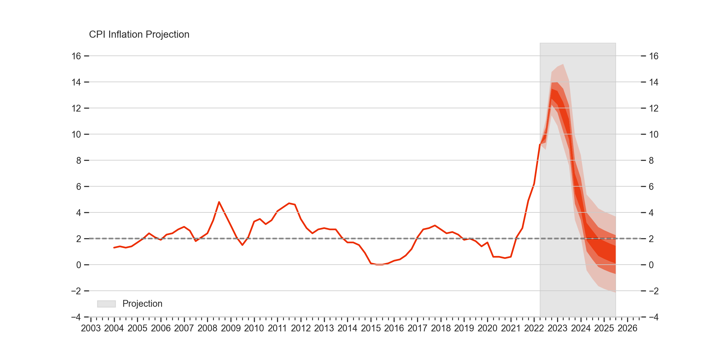
As we can see, this code produces a chart showing:
The historical (observed) values of the CPI inflation from 2004 until a quarter before the projection starts.
Then, the “fan” part is shown in a shadowed area and labeled as projection. This part illustrates the forecasted distribution for 13 quarters from the last observed value.
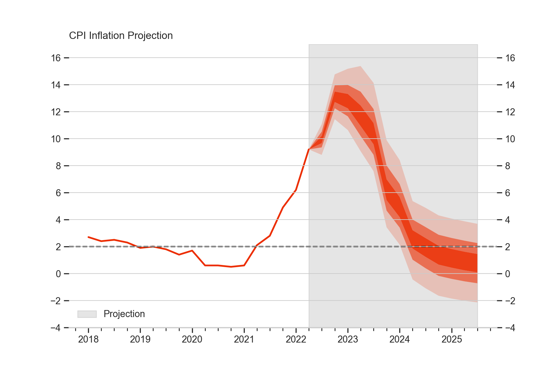
We can restrict the data in the history part to show only the data that we want. For example, in the following fan chart we show only yearly data from 2018.
from fanchart import fan

probs = [0.05, 0.20, 0.35, 0.65,0.80,  0.95]
fan(pars=parameters, probs=probs, historic=history[history.Date >= '2018'])
Single Quarter Fan Charts#
The fanchart package also provides functionality to visualise each of the quarterly forecast on its own.
This is achieved by the function fan_single which requires the following parameters:
loc: Location parameter (Mode)sigma: Uncertainty parametergamma: Skewness parameterprobs: A set probabilities that define the bands in the fan chart.
Important
probs must be a sequence of increasing probabilities in an array type format.
kind: A string either ‘pdf’ or ‘cdf’ to define the type of plot
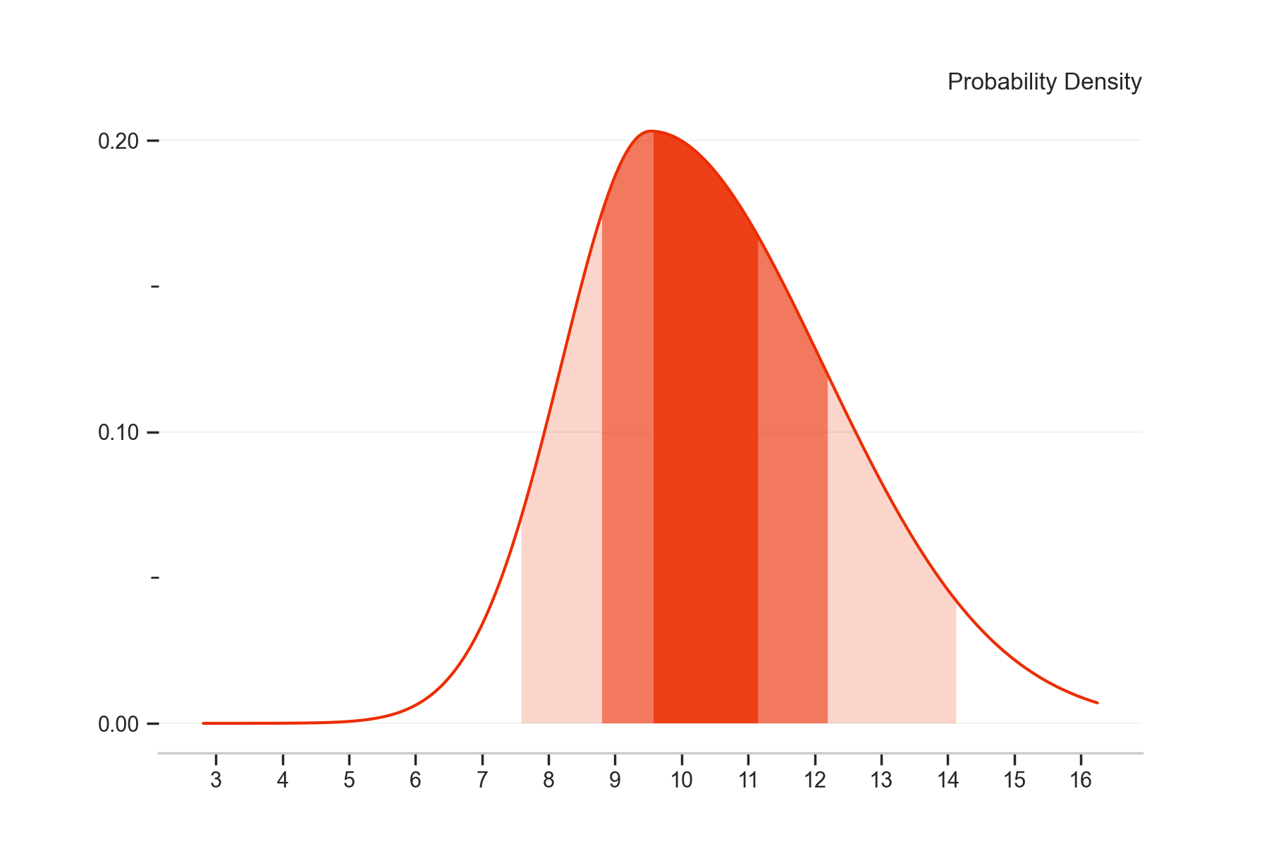
We can plot the forecasted probability density function as follows.
from fanchart import fan_single

probs = [0.05, 0.20, 0.35, 0.65,0.80,  0.95]
fan_single(loc=9.53, sigma=1.68, gamma=1.0, probs=probs, kind='pdf')
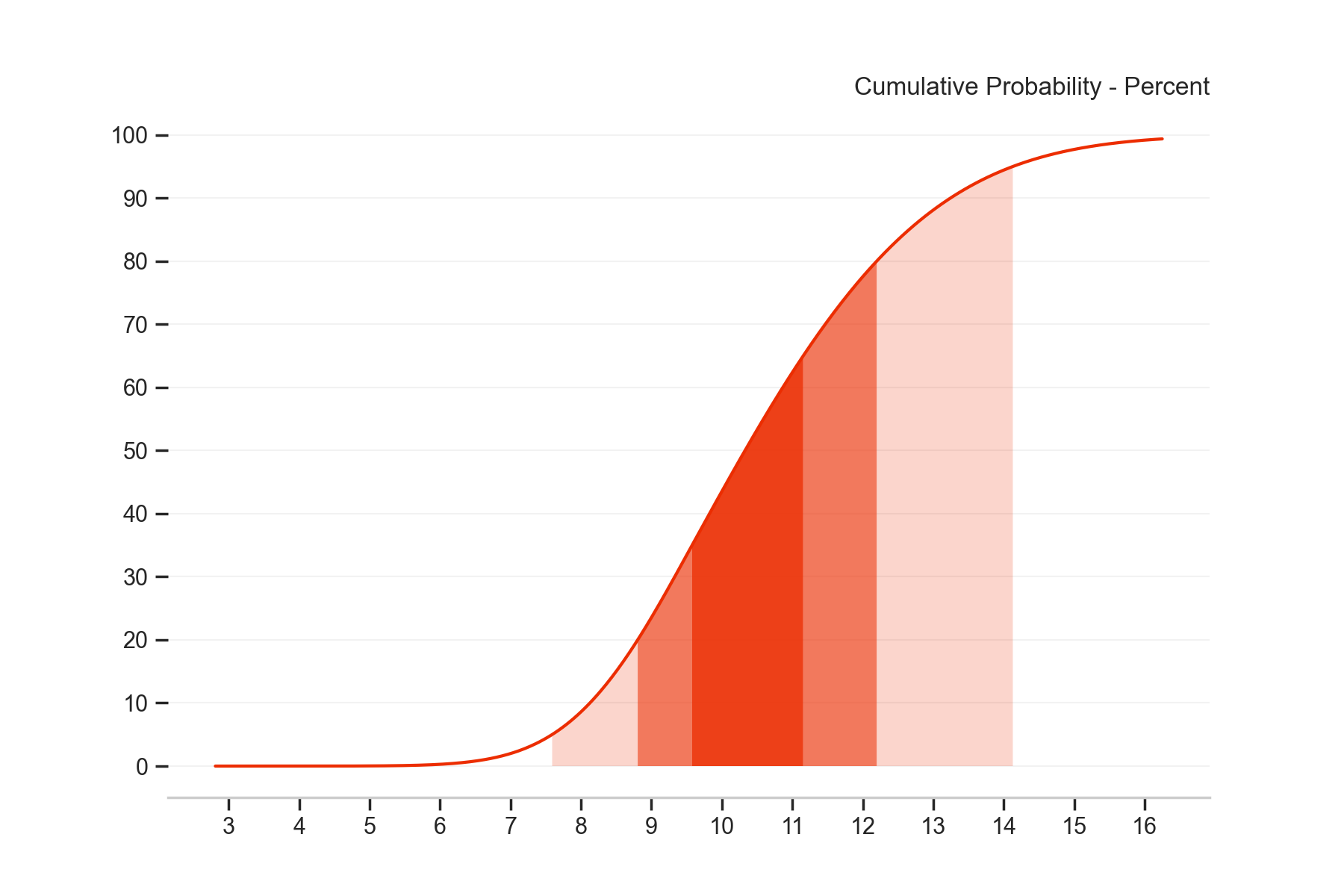
Similarly, we can plot the forecasted cumulative probability function.
from fanchart import fan_single

probs = [0.05, 0.20, 0.35, 0.65,0.80,  0.95]
fan_single(loc=9.53, sigma=1.68, gamma=1.0, probs=probs, kind='cdf')